Safety stock calculation with variable supplier lead time
Last updated: 2026-07-31
Written and reviewed by Seller Profit Guard Editorial Team.
A synthetic SKU averages six units daily with demand deviation two, average lead time eighteen days, lead-time deviation three days, and a 98 percent target. Demand variance contributes seventy-two and timing variance 324; their square root is 19.90 units. Multiplying by z 2.05 gives 40.79, rounded to forty-one units.
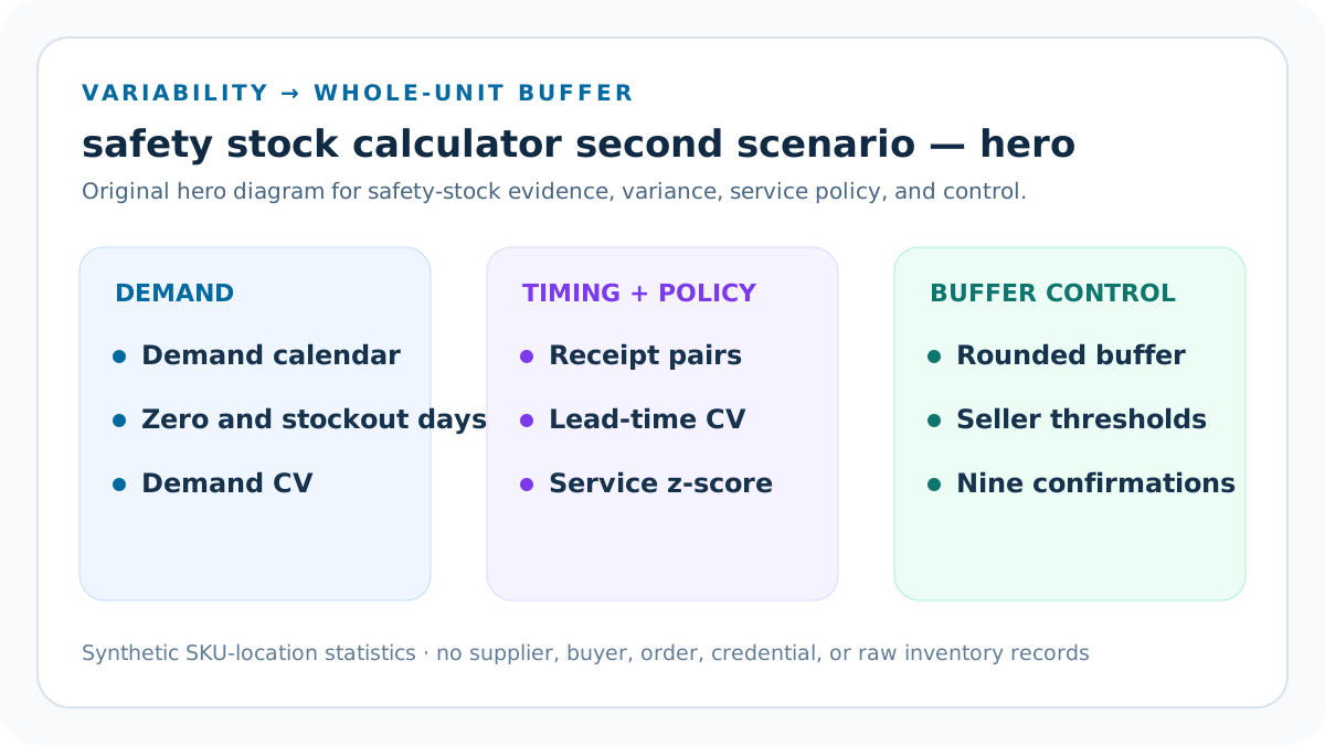
Normalize the 120-day demand history
Keep continuous nonpromotional dates at one item-location grain. The variable-receipt worksheet records the exact source grain, calendar or receipt rule, unit, formula component, timestamp, owner, exception, approval, and preceding accepted value needed for a traceable forty-one-unit buffer.
Do not merge launches or discontinued periods. At review point 1, contrast the nine-unit stable fixture, the forty-one-unit timing-variation fixture, a stockout-censored series, a mixed-receipt defect, and a corrected packet. Identify which output is arithmetic and which conclusion still needs inventory-policy evidence.
Build twelve comparable lead times
Measure from the same start event to usable receipt. The variable-receipt worksheet records the exact source grain, calendar or receipt rule, unit, formula component, timestamp, owner, exception, approval, and preceding accepted value needed for a traceable forty-one-unit buffer.
Split and expedited orders require a rule. At review point 2, contrast the nine-unit stable fixture, the forty-one-unit timing-variation fixture, a stockout-censored series, a mixed-receipt defect, and a corrected packet. Identify which output is arithmetic and which conclusion still needs inventory-policy evidence.
Calculate seventy-two demand variance
Extend daily variance across eighteen average days. The variable-receipt worksheet records the exact source grain, calendar or receipt rule, unit, formula component, timestamp, owner, exception, approval, and preceding accepted value needed for a traceable forty-one-unit buffer.
This component is smaller in the example. At review point 3, contrast the nine-unit stable fixture, the forty-one-unit timing-variation fixture, a stockout-censored series, a mixed-receipt defect, and a corrected packet. Identify which output is arithmetic and which conclusion still needs inventory-policy evidence.
Calculate 324 timing variance
Square six average daily units and three deviation days. The variable-receipt worksheet records the exact source grain, calendar or receipt rule, unit, formula component, timestamp, owner, exception, approval, and preceding accepted value needed for a traceable forty-one-unit buffer.
Timing dominates the variance pool. At review point 4, contrast the nine-unit stable fixture, the forty-one-unit timing-variation fixture, a stockout-censored series, a mixed-receipt defect, and a corrected packet. Identify which output is arithmetic and which conclusion still needs inventory-policy evidence.
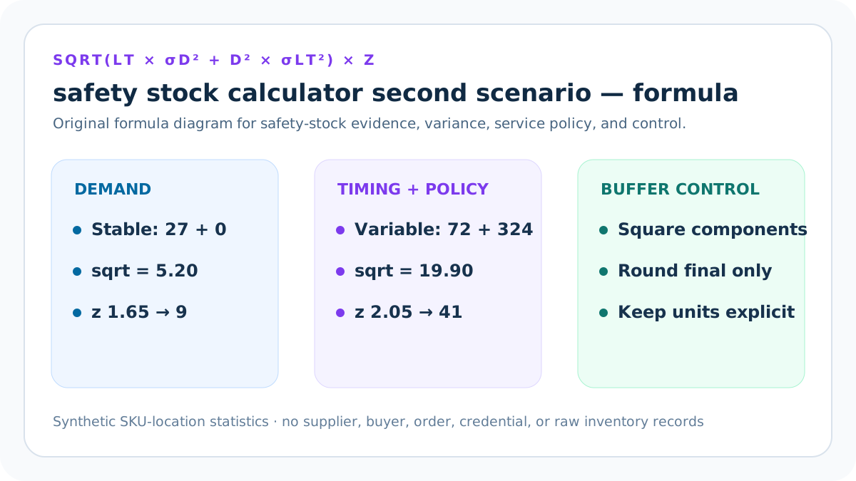
Take the square root of 396
Convert squared uncertainty back to 19.90 units. The variable-receipt worksheet records the exact source grain, calendar or receipt rule, unit, formula component, timestamp, owner, exception, approval, and preceding accepted value needed for a traceable forty-one-unit buffer.
Do not multiply the raw pool by z. At review point 5, contrast the nine-unit stable fixture, the forty-one-unit timing-variation fixture, a stockout-censored series, a mixed-receipt defect, and a corrected packet. Identify which output is arithmetic and which conclusion still needs inventory-policy evidence.
Apply z 2.05 and round
Calculate 40.79 before rounding to forty-one. The variable-receipt worksheet records the exact source grain, calendar or receipt rule, unit, formula component, timestamp, owner, exception, approval, and preceding accepted value needed for a traceable forty-one-unit buffer.
Preserve decimal evidence. At review point 6, contrast the nine-unit stable fixture, the forty-one-unit timing-variation fixture, a stockout-censored series, a mixed-receipt defect, and a corrected packet. Identify which output is arithmetic and which conclusion still needs inventory-policy evidence.
Investigate timing before holding more
Review vendor, lane, location, receipt, and expedite mixtures. The variable-receipt worksheet records the exact source grain, calendar or receipt rule, unit, formula component, timestamp, owner, exception, approval, and preceding accepted value needed for a traceable forty-one-unit buffer.
A larger buffer is not the only remedy. At review point 7, contrast the nine-unit stable fixture, the forty-one-unit timing-variation fixture, a stockout-censored series, a mixed-receipt defect, and a corrected packet. Identify which output is arithmetic and which conclusion still needs inventory-policy evidence.
Safety Stock Example with Variable Lead Time: population integrity control
Record one SKU-location, complete calendar, stable units, availability rules, and effective mappings. Control 1 declares a pass condition, independent reviewer, failure owner, correction deadline, sensitivity test, monitoring signal, and restoration trigger before the proposed buffer can enter a replenishment policy.
Mixed populations are blocked. Apply the control to the concrete variable-receipt worksheet; keep uncertainty buffer separate from expected lead-time demand, reorder point, purchase quantity, and private supplier or order evidence.
Safety Stock Example with Variable Lead Time: demand-distribution control
Retain zero days, stockout flags, exclusions, mean, population deviation, and pattern classification. Control 2 declares a pass condition, independent reviewer, failure owner, correction deadline, sensitivity test, monitoring signal, and restoration trigger before the proposed buffer can enter a replenishment policy.
Observed sales may be censored or non-normal. Apply the control to the concrete variable-receipt worksheet; keep uncertainty buffer separate from expected lead-time demand, reorder point, purchase quantity, and private supplier or order evidence.
Safety Stock Example with Variable Lead Time: receipt-pair control
Retain comparable start and usable-receipt events, sample count, exclusions, average, and population deviation. Control 3 declares a pass condition, independent reviewer, failure owner, correction deadline, sensitivity test, monitoring signal, and restoration trigger before the proposed buffer can enter a replenishment policy.
Supplier timing needs field-level evidence. Apply the control to the concrete variable-receipt worksheet; keep uncertainty buffer separate from expected lead-time demand, reorder point, purchase quantity, and private supplier or order evidence.
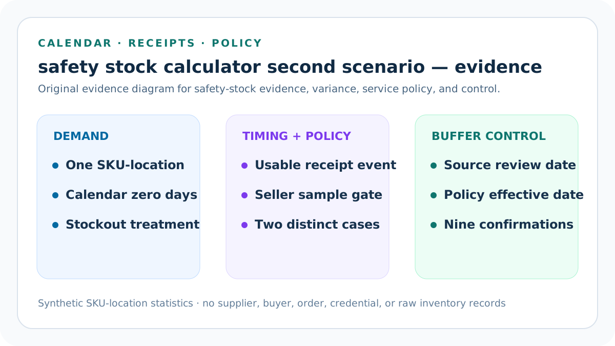
Safety Stock Example with Variable Lead Time: service-policy control
Record the target, z-score mapping, rationale, approver, sensitivity range, and effective period. Control 4 declares a pass condition, independent reviewer, failure owner, correction deadline, sensitivity test, monitoring signal, and restoration trigger before the proposed buffer can enter a replenishment policy.
The tool does not optimize the target. Apply the control to the concrete variable-receipt worksheet; keep uncertainty buffer separate from expected lead-time demand, reorder point, purchase quantity, and private supplier or order evidence.
Safety Stock Example with Variable Lead Time: seller-threshold control
Record the minimum qualifying receipts for Ready and maximum equivalent buffer days; review both scenarios against the same dated policy. Control 5 declares a pass condition, independent reviewer, failure owner, correction deadline, sensitivity test, monitoring signal, and restoration trigger before the proposed buffer can enter a replenishment policy.
A threshold exception requires documented sensitivity rather than silent acceptance. Apply the control to the concrete variable-receipt worksheet; keep uncertainty buffer separate from expected lead-time demand, reorder point, purchase quantity, and private supplier or order evidence.
Safety Stock Example with Variable Lead Time: confirmation and masking control
Confirm all nine scope, calendar, stockout, receipt, service, method, pattern, privacy, and current-rule statements before calculation use. Control 6 declares a pass condition, independent reviewer, failure owner, correction deadline, sensitivity test, monitoring signal, and restoration trigger before the proposed buffer can enter a replenishment policy.
A failed confirmation blocks and masks every derived result. Apply the control to the concrete variable-receipt worksheet; keep uncertainty buffer separate from expected lead-time demand, reorder point, purchase quantity, and private supplier or order evidence.
Safety Stock Example with Variable Lead Time: recovery and privacy control
Keep raw demand and receipts private; retain the prior buffer, monitoring window, stop rule, and restoration authority. Control 7 declares a pass condition, independent reviewer, failure owner, correction deadline, sensitivity test, monitoring signal, and restoration trigger before the proposed buffer can enter a replenishment policy.
Public examples remain synthetic. Apply the control to the concrete variable-receipt worksheet; keep uncertainty buffer separate from expected lead-time demand, reorder point, purchase quantity, and private supplier or order evidence.
Normalize the 120-day demand history: variability lab 1
Reperform the relevant output from the nine-unit and forty-one-unit synthetic cases. Keep continuous nonpromotional dates at one item-location grain. Change one variable only, preserve the remaining population and formula assumptions, list both squared components, and record the expected Block, Review, or Ready classification.
Do not merge launches or discontinued periods. Test an omitted zero day, stockout interval, changed demand window, mismatched receipt, unsupported service target, intermittent pattern, and restored prior buffer. State the protected evidence and operating approval still required.
Build twelve comparable lead times: variability lab 2
Reperform the relevant output from the nine-unit and forty-one-unit synthetic cases. Measure from the same start event to usable receipt. Change one variable only, preserve the remaining population and formula assumptions, list both squared components, and record the expected Block, Review, or Ready classification.
Split and expedited orders require a rule. Test an omitted zero day, stockout interval, changed demand window, mismatched receipt, unsupported service target, intermittent pattern, and restored prior buffer. State the protected evidence and operating approval still required.
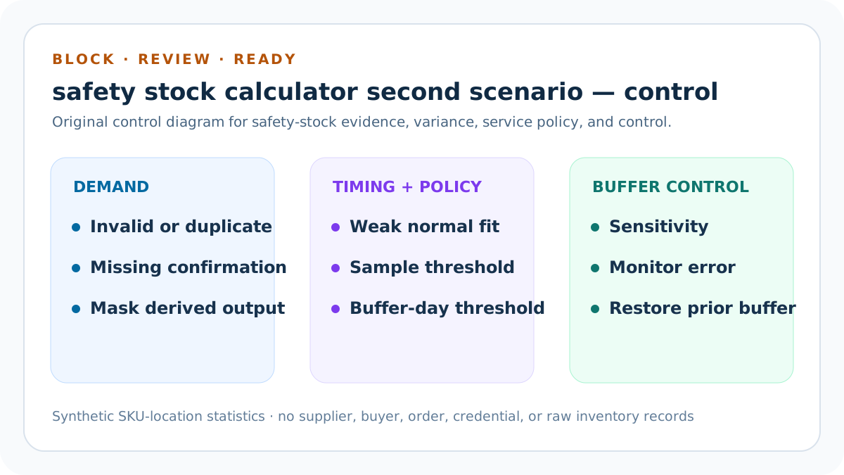
Calculate seventy-two demand variance: variability lab 3
Reperform the relevant output from the nine-unit and forty-one-unit synthetic cases. Extend daily variance across eighteen average days. Change one variable only, preserve the remaining population and formula assumptions, list both squared components, and record the expected Block, Review, or Ready classification.
This component is smaller in the example. Test an omitted zero day, stockout interval, changed demand window, mismatched receipt, unsupported service target, intermittent pattern, and restored prior buffer. State the protected evidence and operating approval still required.
Calculate 324 timing variance: variability lab 4
Reperform the relevant output from the nine-unit and forty-one-unit synthetic cases. Square six average daily units and three deviation days. Change one variable only, preserve the remaining population and formula assumptions, list both squared components, and record the expected Block, Review, or Ready classification.
Timing dominates the variance pool. Test an omitted zero day, stockout interval, changed demand window, mismatched receipt, unsupported service target, intermittent pattern, and restored prior buffer. State the protected evidence and operating approval still required.
Take the square root of 396: variability lab 5
Reperform the relevant output from the nine-unit and forty-one-unit synthetic cases. Convert squared uncertainty back to 19.90 units. Change one variable only, preserve the remaining population and formula assumptions, list both squared components, and record the expected Block, Review, or Ready classification.
Do not multiply the raw pool by z. Test an omitted zero day, stockout interval, changed demand window, mismatched receipt, unsupported service target, intermittent pattern, and restored prior buffer. State the protected evidence and operating approval still required.
Apply z 2.05 and round: variability lab 6
Reperform the relevant output from the nine-unit and forty-one-unit synthetic cases. Calculate 40.79 before rounding to forty-one. Change one variable only, preserve the remaining population and formula assumptions, list both squared components, and record the expected Block, Review, or Ready classification.
Preserve decimal evidence. Test an omitted zero day, stockout interval, changed demand window, mismatched receipt, unsupported service target, intermittent pattern, and restored prior buffer. State the protected evidence and operating approval still required.
Investigate timing before holding more: variability lab 7
Reperform the relevant output from the nine-unit and forty-one-unit synthetic cases. Review vendor, lane, location, receipt, and expedite mixtures. Change one variable only, preserve the remaining population and formula assumptions, list both squared components, and record the expected Block, Review, or Ready classification.
A larger buffer is not the only remedy. Test an omitted zero day, stockout interval, changed demand window, mismatched receipt, unsupported service target, intermittent pattern, and restored prior buffer. State the protected evidence and operating approval still required.
Trace the supplier-timing component in the variable case
The variable fixture uses six average daily units, two units of daily deviation, eighteen average lead-time days, and three days of lead-time deviation. Its demand component is 18 multiplied by two squared, or 72 squared units. Its timing component is six squared multiplied by three squared, or 324 squared units—four and one-half times the demand component.
The square root of the combined 396 is 19.8997 units. Applying the 98 percent mapping of 2.05 gives 40.794 and rounding once gives forty-one. Equivalent buffer days are 6.83, demand coefficient of variation is 33.33 percent, and timing coefficient is 16.67 percent.
Investigate receipt heterogeneity before adding stock
Partition the twelve receipt observations by supplier, fulfillment location, transport mode, expedite status, split receipt, quality hold, and usable-receipt definition. Recalculate only when each partition still represents the same replenishment process; otherwise preserve separate scenarios instead of pooling unlike intervals into a larger deviation.
Compare process remedies with inventory protection: supplier schedule confirmation, earlier order review, smaller but more frequent deliveries, alternate lanes, receiving-capacity changes, or explicit exception handling. The forty-one-unit arithmetic describes entered timing risk and does not choose among those operational responses.
Evidence boundary for a traceable forty-one-unit buffer
The packet can demonstrate entered means, population deviations, coefficients of variation, variance components, combined lead-time demand deviation, service z-score mapping, final multiplication, upward rounding, equivalent days, seller thresholds, nine confirmations, and sensitivity under synthetic inputs.
It cannot prove unconstrained future demand, inventory accuracy, normal-distribution fit, optimal service, supplier performance, carrying affordability, reorder timing, purchase quantity, or stockout prevention.
Release, monitor, and restore the variable-receipt worksheet
Block invalid population, dates, evidence, amounts, samples, duplicate scenarios, service mapping, policy context, missing confirmations, privacy, or open conflicts and mask all derived outputs. Review weak distribution shape, extreme variation, too few receipts for the seller threshold, or excessive equivalent buffer days. Ready clears only the entered statistical worksheet.
Before indexing or operational use, preserve evidence and rollback artifacts, run typecheck, unit, integration, build, content, similarity, SEO, image, link, mobile, strict-route, deployment, and live checks, then compare later error without claiming same-period causality.
Safety Stock Example with Variable Lead Time: concrete working record
The variable worksheet uses 120 calendar days, twelve comparable receipts, average demand 6.00, population daily deviation 2.00, average lead time 18.00, population lead-time deviation 3.00, service target 98 percent, and z 2.05. Demand uncertainty is 18 × 2² = 72 variance units. Receipt-timing uncertainty is 6² × 3² = 324 variance units. The combined pool is 396; its square root is 19.8997 units. Multiply by 2.05 to obtain 40.794 and round up to 41. The 6.83-day equivalent is descriptive only. Supplier constraints and order decisions remain outside.
Sources and further reading
- Seller Profit Guard methodology: Evidence, formula, privacy, correction, release, monitoring, and rollback rules.
- Seller Profit Guard data privacy: Local-first boundaries for SKU, supplier, receipt, order, buyer, and raw inventory data.
- NetSuite Help: Inventory Optimization Calculations: Official demand, lead-time, z-score, safety-stock, rounding, minimum-sample, and approximation formulas.
- NetSuite Help: Inventory Optimization: Official item-location demand, lead-time history, service-level, and planning-value boundary for inventory optimization.
- NetSuite Help: Lead Time and Safety Stock Per Location: Official receipt-derived lead time and location-specific safety-stock context.
- NetSuite Help: Inventory Count: Official inventory-count workflow clarifying why the statistical buffer does not verify on-hand quantity.
- Microsoft Learn: Safety stock fulfillment for items: Official safety-stock planning threshold and replenishment example.
- Microsoft Learn: Planning parameter best practices: Official distinction between safety-stock quantity and safety lead time.
- Microsoft Learn: Planning parameters: Official separation of safety-stock quantity, safety lead time, reorder timing, quantity, and order modifiers.
Related Seller Profit Guard tools
- Safety Stock Calculator: Estimate a statistical SKU-location buffer from demand and lead-time variability.
- Reorder Point Calculator: Use an approved buffer with expected lead-time demand to review a replenishment trigger.
- Variation SKU Generator: Create stable variation identities before location-level analysis.
- SKU Naming Generator: Define the canonical product-variant identity.
- CSV Import Validator: Review a redacted structure before protected data preparation.
- Methodology: Review evidence, formula, privacy, correction, release, and rollback.
- Data Privacy: Protect inventory, supplier, receipt, buyer, credential, and raw export data.
- Safety Stock Formula and Input Rules: Define SKU-location demand, variability, lead-time samples, service z-scores, population formulas, evidence windows, and rounding.
- Safety Stock Worked Example: Stable Lead Time: Calculate a nine-unit buffer from four daily units, 1.50 demand deviation, twelve-day lead time, zero timing deviation, and 95% service.
- Safety Stock Mistakes and Corrections: Correct missing zero days, stockout bias, mixed SKU locations, sample-vs-population errors, weak receipt pairs, z-score misuse, and double buffers.
- Safety Stock Data Sources and Lineage: Map demand calendars, stockouts, order-to-receipt pairs, locations, service targets, formula versions, and policy approvals to authoritative fields.
- Safety Stock Decision and Approval Gates: Separate population validity, statistical fit, service ownership, capacity, carrying exposure, replenishment integration, monitoring, and rollback.
- Stable vs Variable Lead-Time Safety Stock: Compare nine-unit and 41-unit buffers at the same SKU-location grain and isolate demand, receipt-timing, and service-target drivers.
- Weekly Safety Stock Review Routine: Run a repeatable SKU-location cycle for demand calendars, stockouts, receipt pairs, deviations, service policy, sensitivity, exceptions, and restoration.
- How to Interpret Safety Stock Results: Read variance components, combined deviation, z-score, rounded units, equivalent days, and status without claiming optimal service or protection.
- Safety Stock Audit and Change Log: Audit population scope, demand calendars, stockouts, receipt pairs, deviations, service policy, sensitivity, approval, monitoring, and rollback.
Next step: Open Seller Profit Guard.
This is operational planning help, not tax, accounting, legal, financial, or platform-policy advice. Review the Terms and disclaimer, and verify current platform rules and fee assumptions before changing prices.