Stable versus seasonal reorder point comparison

Last updated: 2026-07-31

Written and reviewed by Seller Profit Guard Editorial Team.

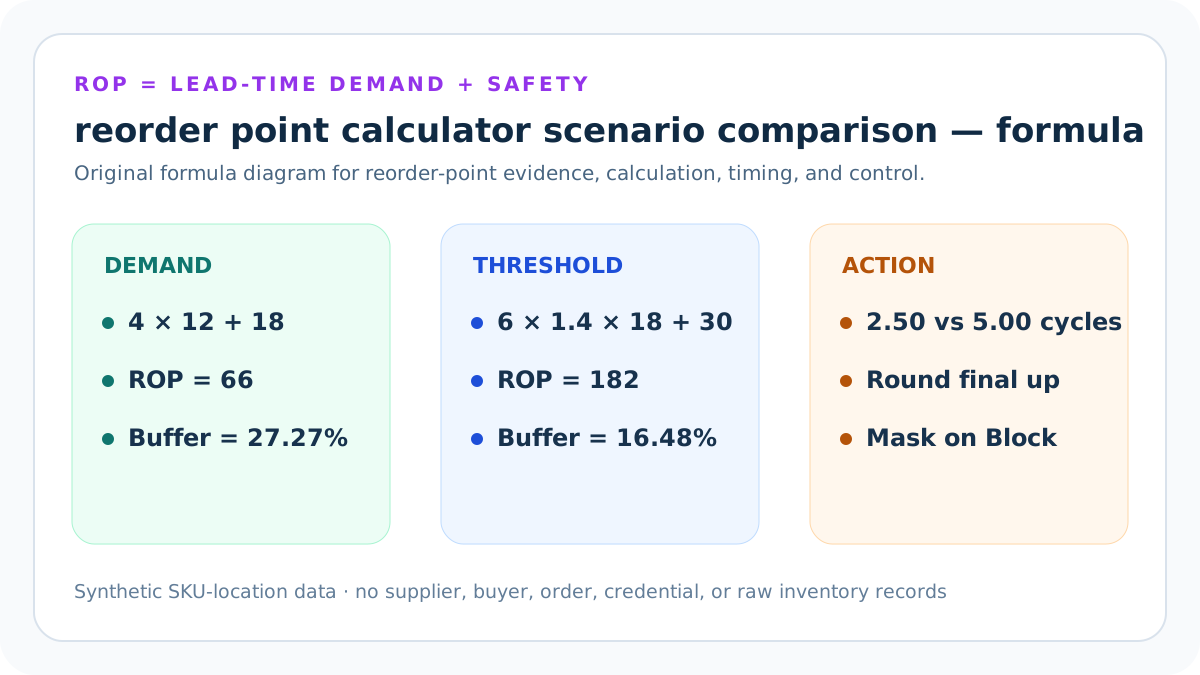
Compare reorder points only after normalizing SKU-location grain, demand unit, review date, inventory-position definition, lead-time evidence, and safety-stock policy. The stable example reaches sixty-six units; the seasonal example reaches 182 because daily demand, lead time, buffer, and multiplier are higher. Difference does not prove either policy is better.

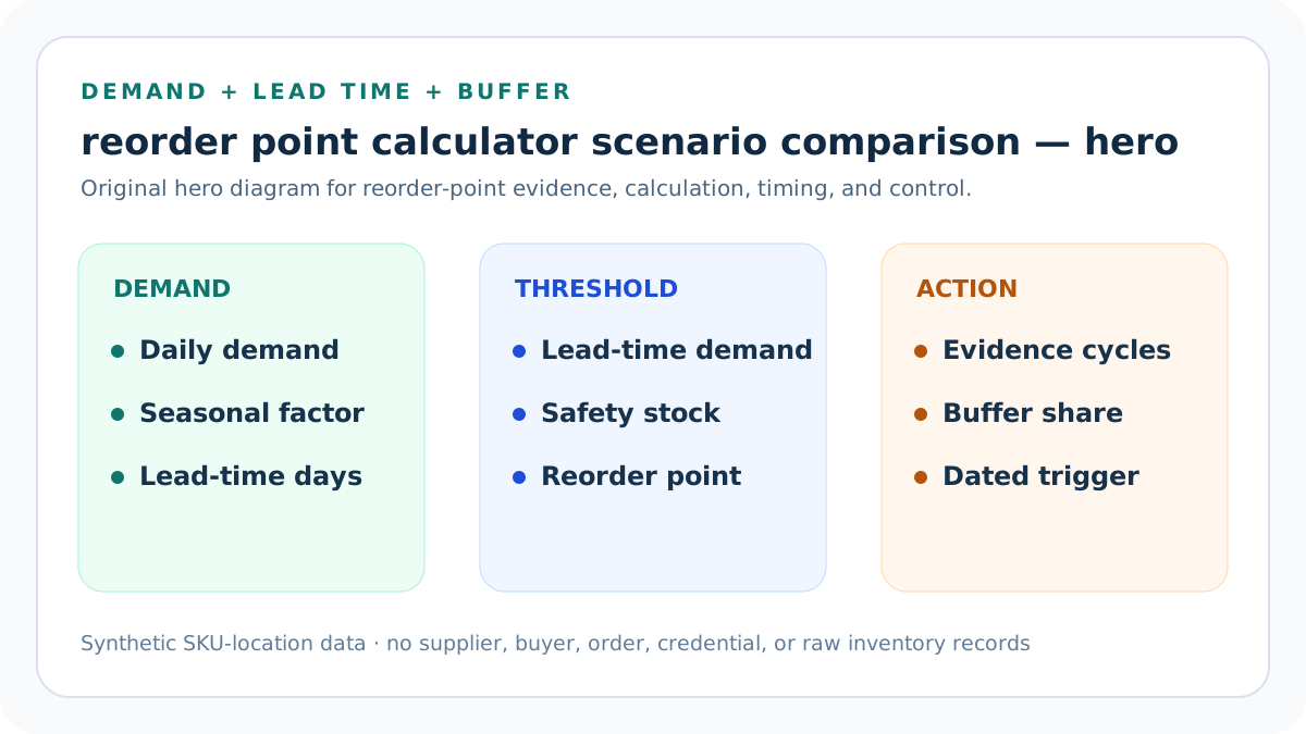
same-grain replenishment comparison from demand and lead time through safety stock, inventory position, threshold, and trigger date — This original diagram explains a driver-based threshold decision with synthetic inventory data.

Normalize the calculation grain

Hold SKU-location, units, and date definitions constant. The same-grain replenishment comparison should retain formula grain, three dated checkpoints, field definition, intermediate calculation, demand-evidence cycles, safety-stock share, seller-owned limits, confirmation status, evidence owner, exception status, approval, and previous value needed for a driver-based threshold decision.

Mixed grain invalidates comparison. At checkpoint 1, compare the stable synthetic worksheet, the seasonal worksheet, a missing-commitment defect, a delayed-receipt case, and a corrected packet. State which part is arithmetic and which part still needs inventory, supplier, purchasing, or receipt evidence.

Compare demand bases

Read direct daily demand against monthly-to-daily conversion. The same-grain replenishment comparison should retain formula grain, three dated checkpoints, field definition, intermediate calculation, demand-evidence cycles, safety-stock share, seller-owned limits, confirmation status, evidence owner, exception status, approval, and previous value needed for a driver-based threshold decision.

Input format changes evidence quality. At checkpoint 2, compare the stable synthetic worksheet, the seasonal worksheet, a missing-commitment defect, a delayed-receipt case, and a corrected packet. State which part is arithmetic and which part still needs inventory, supplier, purchasing, or receipt evidence.

Compare seasonal adjustment

Separate 1.00 from 1.40 and name the event window. The same-grain replenishment comparison should retain formula grain, three dated checkpoints, field definition, intermediate calculation, demand-evidence cycles, safety-stock share, seller-owned limits, confirmation status, evidence owner, exception status, approval, and previous value needed for a driver-based threshold decision.

Multiplier is not performance. At checkpoint 3, compare the stable synthetic worksheet, the seasonal worksheet, a missing-commitment defect, a delayed-receipt case, and a corrected packet. State which part is arithmetic and which part still needs inventory, supplier, purchasing, or receipt evidence.

Compare lead-time exposure

Read twelve days against eighteen receipt-based days. The same-grain replenishment comparison should retain formula grain, three dated checkpoints, field definition, intermediate calculation, demand-evidence cycles, safety-stock share, seller-owned limits, confirmation status, evidence owner, exception status, approval, and previous value needed for a driver-based threshold decision.

Longer exposure raises expected consumption. At checkpoint 4, compare the stable synthetic worksheet, the seasonal worksheet, a missing-commitment defect, a delayed-receipt case, and a corrected packet. State which part is arithmetic and which part still needs inventory, supplier, purchasing, or receipt evidence.

same-grain replenishment comparison: compare lead-time exposure — This original diagram makes a driver-based threshold decision reviewable.

Compare safety-stock policy

Read eighteen units against thirty. The same-grain replenishment comparison should retain formula grain, three dated checkpoints, field definition, intermediate calculation, demand-evidence cycles, safety-stock share, seller-owned limits, confirmation status, evidence owner, exception status, approval, and previous value needed for a driver-based threshold decision.

Buffers reflect separate uncertainty choices. At checkpoint 5, compare the stable synthetic worksheet, the seasonal worksheet, a missing-commitment defect, a delayed-receipt case, and a corrected packet. State which part is arithmetic and which part still needs inventory, supplier, purchasing, or receipt evidence.

Compare position and urgency

Read fourteen units of stable headroom against three seasonal units. The same-grain replenishment comparison should retain formula grain, three dated checkpoints, field definition, intermediate calculation, demand-evidence cycles, safety-stock share, seller-owned limits, confirmation status, evidence owner, exception status, approval, and previous value needed for a driver-based threshold decision.

Urgency depends on inventory too. At checkpoint 6, compare the stable synthetic worksheet, the seasonal worksheet, a missing-commitment defect, a delayed-receipt case, and a corrected packet. State which part is arithmetic and which part still needs inventory, supplier, purchasing, or receipt evidence.

Choose a supported policy

Use observed forecast error and supplier evidence. The same-grain replenishment comparison should retain formula grain, three dated checkpoints, field definition, intermediate calculation, demand-evidence cycles, safety-stock share, seller-owned limits, confirmation status, evidence owner, exception status, approval, and previous value needed for a driver-based threshold decision.

A larger threshold is not automatically safer. At checkpoint 7, compare the stable synthetic worksheet, the seasonal worksheet, a missing-commitment defect, a delayed-receipt case, and a corrected packet. State which part is arithmetic and which part still needs inventory, supplier, purchasing, or receipt evidence.

Stable vs Seasonal Reorder Points Compared: grain and definition control

Record one SKU, location, unit, inventory-field map, inventory review date, official-source review date, policy effective date, and timezone. Control 1 declares the exact source, unit, date, pass condition, reviewer, failure owner, correction deadline, and restoration trigger before the threshold can influence an alert or purchasing review.

Mixed grains, impossible dates, and future-effective evidence are blocked. Apply this control to the concrete same-grain replenishment comparison; keep reorder point separate from purchase quantity, projected trigger separate from delivery or stockout date, and aggregate public evidence separate from private SKU, supplier, and order records.

Stable vs Seasonal Reorder Points Compared: demand and stockout control

Retain the demand window, lead-time-cycle coverage, exclusions, unavailable days, raw rate, seasonal factor, and event scope. Control 2 declares the exact source, unit, date, pass condition, reviewer, failure owner, correction deadline, and restoration trigger before the threshold can influence an alert or purchasing review.

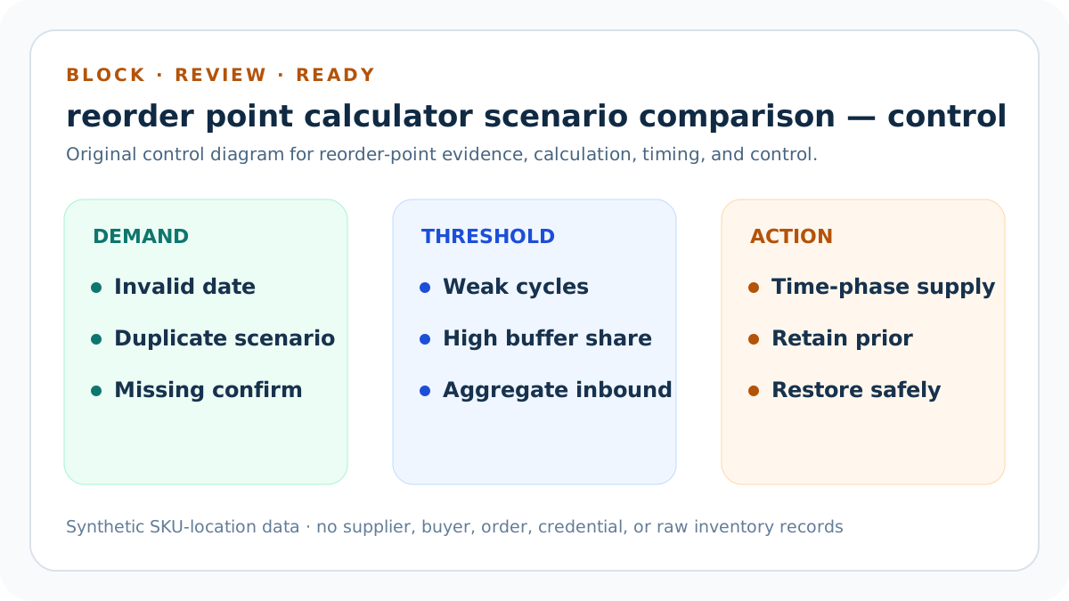
Observed sales can be constrained, and weak cycle coverage moves to Review. Apply this control to the concrete same-grain replenishment comparison; keep reorder point separate from purchase quantity, projected trigger separate from delivery or stockout date, and aggregate public evidence separate from private SKU, supplier, and order records.

Stable vs Seasonal Reorder Points Compared: lead-time and buffer control

Pair recognition dates with usable receipts, keep approved safety stock separate, and compare its share of reorder point with the seller-owned maximum. Control 3 declares the exact source, unit, date, pass condition, reviewer, failure owner, correction deadline, and restoration trigger before the threshold can influence an alert or purchasing review.

Promises, buffers, and review thresholds require named owners. Apply this control to the concrete same-grain replenishment comparison; keep reorder point separate from purchase quantity, projected trigger separate from delivery or stockout date, and aggregate public evidence separate from private SKU, supplier, and order records.

same-grain replenishment comparison: stable vs seasonal reorder points compared: lead-time and buffer control — This original diagram makes a driver-based threshold decision reviewable.

Stable vs Seasonal Reorder Points Compared: position and timing control

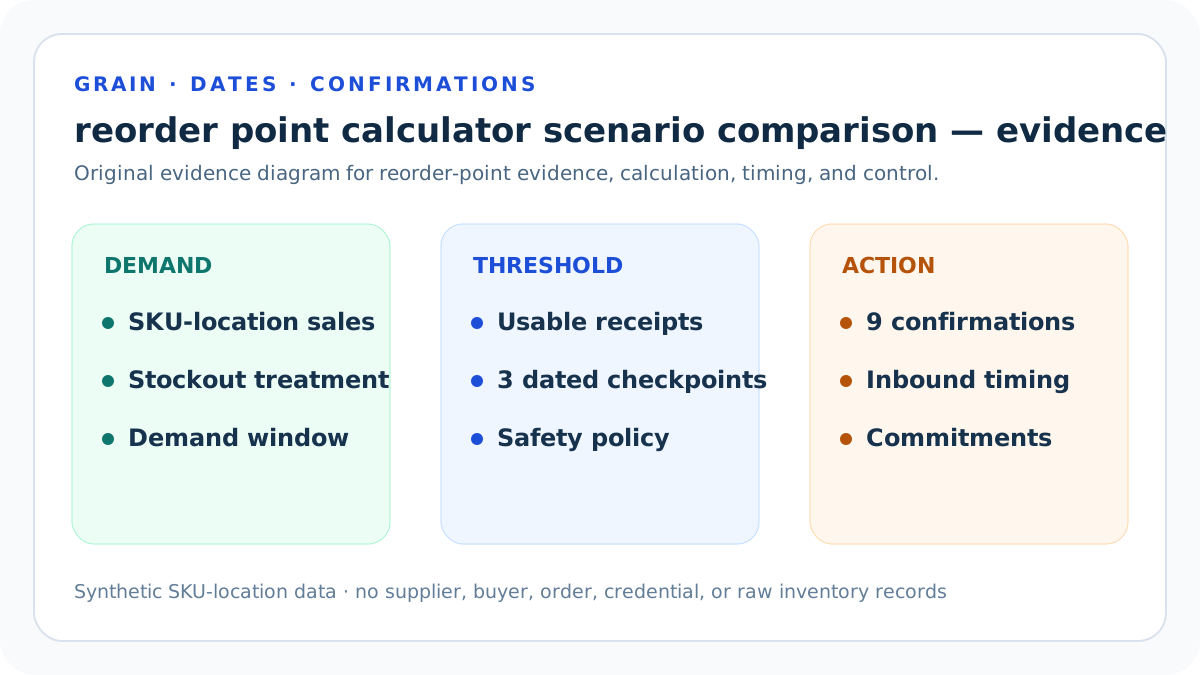
Reconcile on hand, eligible inbound, commitments, transfers, holds, time-phased availability, and the nine evidence confirmations. Control 4 declares the exact source, unit, date, pass condition, reviewer, failure owner, correction deadline, and restoration trigger before the threshold can influence an alert or purchasing review.

Aggregate totals can hide timing defects, while missing confirmations block outputs. Apply this control to the concrete same-grain replenishment comparison; keep reorder point separate from purchase quantity, projected trigger separate from delivery or stockout date, and aggregate public evidence separate from private SKU, supplier, and order records.

Stable vs Seasonal Reorder Points Compared: privacy and recovery control

Keep raw inventory and purchasing records private; retain two materially distinct scenarios, the prior threshold, alert, approval, stop rule, and restoration packet. Control 5 declares the exact source, unit, date, pass condition, reviewer, failure owner, correction deadline, and restoration trigger before the threshold can influence an alert or purchasing review.

Public evidence remains synthetic and duplicate scenarios are rejected. Apply this control to the concrete same-grain replenishment comparison; keep reorder point separate from purchase quantity, projected trigger separate from delivery or stockout date, and aggregate public evidence separate from private SKU, supplier, and order records.

Normalize the calculation grain: replenishment exercise 1

Recalculate the relevant result from the 66-unit stable threshold and the 182-unit seasonal threshold. Hold SKU-location, units, and date definitions constant. Also reproduce the 2.50 versus 5.00 demand-evidence cycles and the 27.27% versus 16.48% safety-stock shares. Change one input only, preserve all other assumptions, list the affected intermediate values, and record the expected Block, Review, or Ready state.

Mixed grain invalidates comparison. The exercise should test a stockout-distorted demand window, stale lead time, missing commitment, ineligible inbound receipt, changed safety stock, seasonal event, and restored prior threshold. Name the external inventory and purchasing evidence still required.

Compare demand bases: replenishment exercise 2

Recalculate the relevant result from the 66-unit stable threshold and the 182-unit seasonal threshold. Read direct daily demand against monthly-to-daily conversion. Also reproduce the 2.50 versus 5.00 demand-evidence cycles and the 27.27% versus 16.48% safety-stock shares. Change one input only, preserve all other assumptions, list the affected intermediate values, and record the expected Block, Review, or Ready state.

Input format changes evidence quality. The exercise should test a stockout-distorted demand window, stale lead time, missing commitment, ineligible inbound receipt, changed safety stock, seasonal event, and restored prior threshold. Name the external inventory and purchasing evidence still required.

Compare seasonal adjustment: replenishment exercise 3

Recalculate the relevant result from the 66-unit stable threshold and the 182-unit seasonal threshold. Separate 1.00 from 1.40 and name the event window. Also reproduce the 2.50 versus 5.00 demand-evidence cycles and the 27.27% versus 16.48% safety-stock shares. Change one input only, preserve all other assumptions, list the affected intermediate values, and record the expected Block, Review, or Ready state.

Multiplier is not performance. The exercise should test a stockout-distorted demand window, stale lead time, missing commitment, ineligible inbound receipt, changed safety stock, seasonal event, and restored prior threshold. Name the external inventory and purchasing evidence still required.

Compare lead-time exposure: replenishment exercise 4

Recalculate the relevant result from the 66-unit stable threshold and the 182-unit seasonal threshold. Read twelve days against eighteen receipt-based days. Also reproduce the 2.50 versus 5.00 demand-evidence cycles and the 27.27% versus 16.48% safety-stock shares. Change one input only, preserve all other assumptions, list the affected intermediate values, and record the expected Block, Review, or Ready state.

Longer exposure raises expected consumption. The exercise should test a stockout-distorted demand window, stale lead time, missing commitment, ineligible inbound receipt, changed safety stock, seasonal event, and restored prior threshold. Name the external inventory and purchasing evidence still required.

same-grain replenishment comparison: compare lead-time exposure: replenishment exercise 4 — This original diagram makes a driver-based threshold decision reviewable.

Compare safety-stock policy: replenishment exercise 5

Recalculate the relevant result from the 66-unit stable threshold and the 182-unit seasonal threshold. Read eighteen units against thirty. Also reproduce the 2.50 versus 5.00 demand-evidence cycles and the 27.27% versus 16.48% safety-stock shares. Change one input only, preserve all other assumptions, list the affected intermediate values, and record the expected Block, Review, or Ready state.

Buffers reflect separate uncertainty choices. The exercise should test a stockout-distorted demand window, stale lead time, missing commitment, ineligible inbound receipt, changed safety stock, seasonal event, and restored prior threshold. Name the external inventory and purchasing evidence still required.

Compare position and urgency: replenishment exercise 6

Recalculate the relevant result from the 66-unit stable threshold and the 182-unit seasonal threshold. Read fourteen units of stable headroom against three seasonal units. Also reproduce the 2.50 versus 5.00 demand-evidence cycles and the 27.27% versus 16.48% safety-stock shares. Change one input only, preserve all other assumptions, list the affected intermediate values, and record the expected Block, Review, or Ready state.

Urgency depends on inventory too. The exercise should test a stockout-distorted demand window, stale lead time, missing commitment, ineligible inbound receipt, changed safety stock, seasonal event, and restored prior threshold. Name the external inventory and purchasing evidence still required.

Choose a supported policy: replenishment exercise 7

Recalculate the relevant result from the 66-unit stable threshold and the 182-unit seasonal threshold. Use observed forecast error and supplier evidence. Also reproduce the 2.50 versus 5.00 demand-evidence cycles and the 27.27% versus 16.48% safety-stock shares. Change one input only, preserve all other assumptions, list the affected intermediate values, and record the expected Block, Review, or Ready state.

A larger threshold is not automatically safer. The exercise should test a stockout-distorted demand window, stale lead time, missing commitment, ineligible inbound receipt, changed safety stock, seasonal event, and restored prior threshold. Name the external inventory and purchasing evidence still required.

Evidence boundary for a driver-based threshold decision

The packet can demonstrate entered demand normalization, seasonal multiplication, lead-time extension, safety-stock addition, whole-unit rounding, demand-evidence-cycle coverage, safety-stock share, declared inventory-position arithmetic, headroom, and a straight-line trigger date under two distinct synthetic inputs.

It cannot forecast unconstrained demand, prove inventory accuracy or exact receipt timing, choose an optimal buffer or order quantity, reserve cash or capacity, place a purchase order, guarantee supplier performance, or prevent stockouts.

Release, monitor, and restore the same-grain replenishment comparison

Block invalid scope, real dates, demand, lead time, safety stock, inventory fields, thresholds, scenario distinction, confirmations, privacy, or open conflicts, and mask every derived result. Review short histories, weak evidence-cycle coverage, high safety-stock share, extreme seasonal adjustments, and aggregate inbound timing. Ready clears only the entered simple model.

Before indexing or operational use, retain source and rollback artifacts, run typecheck, unit, integration, build, content, similarity, SEO, image, link, mobile, strict-404, deployment, and live checks, then measure delayed discovery and later planning error without claiming same-period causality.

Stable vs Seasonal Reorder Points Compared: concrete working record

Place both scenarios in a driver table: demand input basis, normalized daily demand, seasonality multiplier and event dates, adjusted daily demand, lead-time days and receipt sample, lead-time demand, safety stock, on hand, eligible inbound, commitments, inventory position, reorder point, headroom, trigger days, and trigger date. Then calculate the contribution of each driver to the 116-unit threshold difference without claiming causality. The stable case is 4 × 12 + 18 = 66. The seasonal case is ceil(6 × 1.40 × 18 + 30) = 182. Review policy suitability with later observed error and operating constraints.

Sources and further reading

Seller Profit Guard methodology: Evidence, formula, privacy, correction, release, and rollback rules.
Seller Profit Guard data privacy: Local-first boundaries for inventory, supplier, order, buyer, and raw catalog data.
Shopify Help: Low stock: Official lead-time and sales-per-day reorder-point example, depletion context, and Stocky retirement notice.
Microsoft Learn: Handling reordering policies: Official projected-inventory, safety-stock, time-bucket, and replenishment-policy boundaries.
Microsoft Learn: Reordering policy best practices: Official boundary between replenishment timing, quantity, and order modifiers.
NetSuite Help: Inventory Optimization: Official item-location demand history, service-level, and lead-time variability context.
NetSuite Help: Lead Time and Safety Stock Per Location: Official receipt-derived lead-time and location-specific safety-stock context.
Microsoft Learn: Inventory Availability report: Official on-hand, expected supply, demand, purchase-order, transfer, and SKU availability boundaries.
Square Support: Create inventory alerts: Official location-level low-stock threshold and alert behavior.

Related Seller Profit Guard tools

Reorder Point Calculator: Calculate lead-time demand, safety-stock threshold, inventory position, and trigger date.
Variation SKU Generator: Create stable variation identities before location-level replenishment planning.
SKU Naming Generator: Define a canonical product-variant identity.
Listing Cost Library Calculator: Keep inventory thresholds separate from product-cost evidence.
CSV Import Validator: Review a redacted file structure before private inventory work.
Methodology: Review evidence, formula, privacy, correction, release, and rollback.
Data Privacy: Protect inventory, supplier, order, buyer, credential, and raw export data.
Reorder Point Formula and Input Rules: Define SKU-location demand, lead time, safety stock, inventory position, seasonality, evidence, and trigger-date assumptions.
Reorder Point Worked Example: Stable Demand: Calculate a 66-unit reorder point and dated trigger for a stable SKU with four daily units, twelve lead-time days, and safety stock.
Seasonal Reorder Point Worked Example: Convert monthly demand, apply a 1.40 seasonal factor, and calculate a 182-unit threshold for a longer replenishment lead time.
Reorder Point Mistakes That Cause Stockouts: Correct mixed locations, sales-window bias, missing commitments, false inbound, stale lead time, double-counted buffers, and wrong date labels.
Reorder Point Data Sources and Evidence: Source SKU-location demand, stockouts, receipts, safety stock, on hand, inbound, commitments, supplier rules, and inventory policy evidence.
Reorder Point Decision and Release Gates: Separate data-validity, model, trigger, time-phased receipt, purchasing, approval, monitoring, rollback, and exception gates.
Weekly Reorder Point Review Routine: Run a repeatable SKU-location review for counts, commitments, receipts, demand windows, safety stock, alerts, exceptions, and restoration.
How to Interpret Reorder Point Results: Read lead-time demand, safety stock, inventory position, headroom, trigger days, and status without claiming forecast or order proof.
Reorder Point Audit and Change Log: Audit SKU-location grain, demand, lead time, safety stock, inventory position, trigger, purchasing action, monitoring, and restoration.

Next step: Open Seller Profit Guard.

This is operational planning help, not tax, accounting, legal, financial, or platform-policy advice. Review the Terms and disclaimer, and verify current platform rules and fee assumptions before changing prices.